Part I: From Vectors to Functions

What are operators, and why should neural networks learn them?

What Is an Operator?

Example: $u_0(x) \mapsto u(x, T)$: given an initial temperature distribution, predict the temperature at time $T$.

Why Functions, Not Vectors?

A vector $[u_1, u_2, \ldots, u_n]$ is just a discretization of a function $u(x)$ on a grid.

If we think in terms of functions, the learned operator should work at any resolution: coarse or fine.

This is fundamentally different from CNNs, which are tied to a fixed grid resolution.

Universal Approximation for Operators

Chen & Chen (1995): A neural network with a single hidden layer can approximate any continuous nonlinear operator. [paper]

$$\mathcal{G}(u)(y) \approx \sum_{i=1}^{p} c_i(u) \cdot \psi_i(y)$$

$c_i(u)$ , coefficients from the input function (the branch)
$\psi_i(y)$ , basis functions at the query point (the trunk)

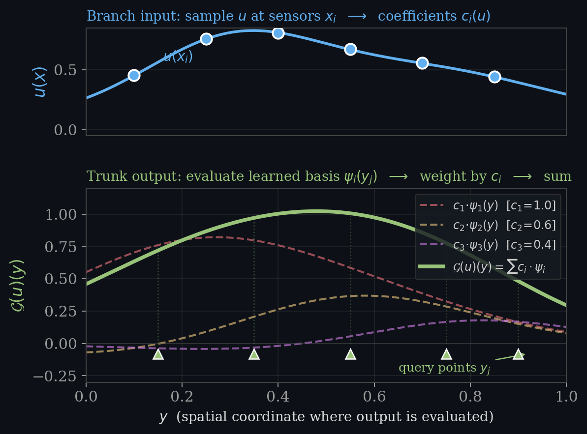
This is a modal decomposition: basis functions $\times$ coefficients, summed. It is the theoretical foundation for DeepONet.

The Operator Learning Setup

Part II: Deep Operator Networks

From classical modal decomposition to learned operators.

Spatial-Temporal Modal Decomposition

Many PDE solutions can be written as a sum of spatial modes weighted by temporal coefficients:

DeepONet Architecture

Two sub-networks whose outputs are combined via a dot product (Lu et al., Nature Machine Intelligence, 2021): [paper]

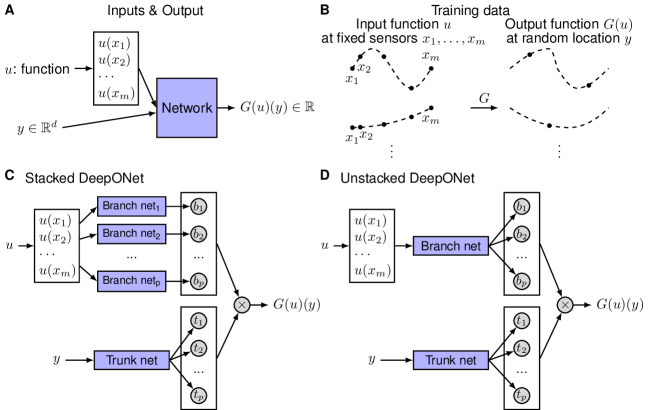
DeepONet = Learned Modal Decomposition

Training DeepONet

Physics-informed (PI-DeepONet): add PDE residual loss where $f$ is the forcing/source term:

DeepONet: Key Properties

DeepONet: Results

From Lu et al. (2021), DeepONet achieves high accuracy across diverse PDE families:

Lu et al. (2021). Learning nonlinear operators via DeepONet. Nature Machine Intelligence, 3, 218–229. [link]

Part III: Green's Functions → Fourier Neural Operators

From integral solutions to learnable spectral layers.

Green's Functions: The Integral Solution

Superposition: Interactive

For the 1D diffusion equation $\;\frac{\partial u}{\partial t} = \nu \frac{\partial^2 u}{\partial x^2} + f(x)$, the Green's function is a Gaussian kernel. Add impulses to $f(x)$ and see the superposition build the solution $u(x)$.

From Green's Functions to Neural Operator Layers

Green's functions rely on linearity (superposition). For nonlinear PDEs, no simple $G$ exists. But we can learn a kernel and compose it through nonlinear layers.

Kovachki, N. et al. (2023). Neural Operator: Learning Maps Between Function Spaces. JMLR, 24(89), 1–97.

The Convolution Trick

A general kernel $\kappa(x, y)$ is expensive: $O(n^2)$ to evaluate on a grid of $n$ points.

Assume translation invariance: the kernel depends only on the difference $\kappa(x, y) = \kappa(x - y)$.

→ This is convolution!

→ Convolution in space = multiplication in Fourier domain.

FNO Layer: Interactive

Each Fourier Neural Operator layer: apply FFT, multiply by learned weights, inverse FFT, add spatial path, activate.

FNO: Key Properties

Li, Z., Kovachki, N., Azizzadenesheli, K., Liu, B., Bhatt, K., Stuart, A. & Anandkumar, A. (2021). Fourier Neural Operator for Parametric PDEs. ICLR 2021.

In Code: DeepONet

class DeepONet(nn.Module):
    def __init__(self, u_dim, y_dim, p=64):
        super().__init__()
        self.branch = nn.Sequential(        # input function → coefficients
            nn.Linear(u_dim, 128), nn.ReLU(),
            nn.Linear(128, p))
        self.trunk = nn.Sequential(         # query point → basis functions
            nn.Linear(y_dim, 128), nn.ReLU(),
            nn.Linear(128, p))

    def forward(self, u, y):
        b = self.branch(u)                  # (batch, p)
        t = self.trunk(y)                   # (batch, p)
        return (b * t).sum(-1)              # dot product

In Code: FNO Layer

class SpectralConv1d(nn.Module):
    def __init__(self, ch, modes):
        super().__init__()
        self.modes = modes
        self.weights = nn.Parameter(         # learnable Fourier weights
            torch.randn(ch, ch, modes, 2))

    def forward(self, x):                    # x: (batch, ch, N)
        x_ft = torch.fft.rfft(x)
        out_ft = torch.zeros_like(x_ft)
        out_ft[:,:,:self.modes] = \          # multiply low modes by R
            complex_mul(x_ft[:,:,:self.modes], self.weights)
        return torch.fft.irfft(out_ft, n=x.size(-1))

Part IV: Comparing Architectures

DeepONet vs FNO vs PINNs: when to use what.

When to Use What

Other Operator Architectures

The field is evolving rapidly. Some notable variants:

Connections Across the Course

Summary: Design Principles

References